Diogenes, the sampler from Sinope

Although I graduated long ago from inmate to guard, I benefit from continued receipt of the American Statistical Society’s student magazine. Well, benefit – when one is more than a decade an Econometrician (of varying skill and/or pedigree) there isn’t much to be had inside.

Except, that is, for the likes of this (click for a larger/readable version):

Very amusing. Fair to say – Diogenes should have invested a little time, first, searching for some decent help with survey design.

One did not need a computer to predict the decline of quantitative management

The amount of money managed by so-called quant funds has dropped by up to 40 per cent in the past six months, as the drawbacks of the once rapidly growing strategy have been laid bare by the credit market turmoil.

Quantitative management, which uses computer models to make trading decisions, is behind the success of some of the best known hedge funds and institutional managers. Some estimates pegged the amount managed this way at about $500bn before the slump hit.

However, those using the strategies concede that they were unaware of how popular quant investing had become, and how many quant managers were doing the same trades. As a result, managers deleveraging in times of market turmoil would exit the same trading positions as many other managers, resulting in sharp losses for several previously high-flying funds.

Is commentary even needed, here? Deterministic trading methods were shown to be pretty garbage back when I did my two (utterly wasted) undergraduate semesters in Finance. In fact I learned more from Econometrics than Finance (precisely why quantitative skills are so important!). I’m sure these computer programmes are making quite sophisticated decisions, but when many others are making the same decisions, those trades become enormously foolish ones, timing-wise.

“… fundamental errors in methodology and even in basic calculations”

The state of Alaska said on Thursday it was suing Mercer for more than $1.8bn, accusing the unit of Marsh & McLennan of making errors in calculating pension plans’ expected liabilities.

The lawsuit filed on Thursday in state superior court in Juneau accuses Mercer of mistaken assumptions and methods about future healthcare costs and basic mathematical and technical errors.

“Fully aware of the billions of dollars at stake, Mercer nevertheless made fundamental errors in methodology and even in basic calculations, and failed to assign competent, experienced personnel to work for the plans,” the lawsuit charges.

“Because of this misconduct, Mercer miscalculated – by over $1.8bn – the contributions necessary to fund the (pension) plans.”

Ooh, that smarts.

I’ve been pondering since this morning, what’s up with this heat?

Near-gratuitous One Piece reference (watch every episode here!). One Piece is awesome. Make a note. Awesome.

So. Today’s weather:

Walking around with the missus (we went to Grant’s tomb – boring, but, in their defence, closed for the holiday. Still), she commented on the heat, its unseasonality, how freezing cold it had been in her youth, etc. Honestly, she should have known better – a statistician and a contrarian for a husband? Crazy idea.

My counter-arguments: (1) that the temperature on the day of Thanksgiving is a variable, like any other. The week of Thanksgiving, maybe. But the day? Temperature and time both are continuous variables. A single day is just way too precise to pin something like that on; (2) my wife was probably remembering particularly cold days from her youth, which was affecting her memory of the true average temperatures for this period.

So, being the manner of econometrician that I am. After dinner, I jumped on the web and started looking. I found my way to Almanac.com, and started pulling out the temperature for all of the November 22nds since the birth of my wife (1981; a fine year for pretty girls).

I had to jump from Central Park to JFK in 1994 (no Central Park data past then, but I checked a handful of the dates since, and there’s no apparent measurement problem). Descriptive statistics:

So, what do I do? I start looking for 60 degrees (today’s) in the 95% Confidence Interval for the mean temperature on Thanksgiving Day.

$ latex begin{eqnarray*}
95\%CI_{\mu } &=&\overline{x}\pm t_{.025,26}\times \sigma _{\overline{x}} \\
&=&\overline{x}\pm t_{.025,26}\times \frac{\sigma }{\sqrt{n}} \\
&=&45.4\pm 2.056\times 1.76 \\
&=&41.78\text{ to }49
\end{eqnarray*} $

WordPress’ latex plug-in is ass. It was supposed to look like this:

So today’s 60 degrees just (just) misses out. Like fun it does.

The conclusion: Confidence Interval conclusions can vary, but we can say that, for example, 95% of Thanksgivings will not have a mean temperature of 60 degrees (97.5% of them will be less than 60 degrees – by a long way). We are 95% certain that the population mean (the true mean for Thanksgiving Day) is not 60 degrees.

Is today’s temperature therefore extreme? We can visit the 99% confidence interval:

$ latex begin{eqnarray*}
99\%CI_{\mu } &=&\overline{x}\pm t_{.005,26}\times \sigma _{\overline{x}} \\
&=&\overline{x}\pm t_{.005,26}\times \frac{\sigma }{\sqrt{n}} \\
&=&45.4\pm 2.779\times 1.76 \\
&=&40.51\text{ to }50.29
\end{eqnarray*} $

Or, again,

Again, um, just? Barely. There is less than a 1% chance that, on any given Thanksgiving Day, the mean temperature will be this far from the average (and less than half of one percent that it will be this high). Statistically, it was an extreme event.

There is far less than a 1% chance: the p-value for an average temperature of 60 degrees is, in fact, basically 0 (the t-statistic being 8.3)

I managed a partial victory. The two lowest days – and the only two below 30 degrees – occurred in my wife’s youth, and the lowest occurred the year she was freezing cold out in the parade itself. So I scored a minor point.

A caveat is the mean. I used the entire series. This is to say, a caveat to the numbers – that result isn’t going anywhere.

Suppose I used only the Thanksgivings up until this one? Today’s was the maximum for the series: the next highest was 59 degrees. Cutting out today’s 60 degrees lowers the average to 44.8, and the standard deviation to 8.84. It also lowers the sample size, increasing the “critical value” t-statistic slightly (due to the lower degrees of freedom) as well as the standard error. The new 99% Confidence interval narrows, slightly, but also shifts downwards: 40 degrees to 49.6. Either way, 60 degrees (new t-statistic 8.77) is still nowhere near likely to be another average temperature in a hurry.

Hannah Montana fan club members to sue the fan club. Hopefully the judge is a Bayesian

This is a re-post. For some reason pieces of the original did not upload and I was too tired to even check. This morning I added the regression stuff.

While I’m in the mood to update old stories: here’s the latest one about Hannah Montana

Thousands of “Hannah Montana” fans who couldn’t get concert tickets could potentially join a lawsuit against the teen performer’s fan club over memberships they claim were supposed to give them priority for seats.

The lawsuit was filed on behalf of a New Jersey woman and anyone else who joined the Miley Cyrus Fan Club based on its promise that joining would make it easier to get concert tickets from the teen star’s Web site.

…

“They deceptively lured thousands of individuals into purchasing memberships into the Miley Cyrus Fan Club,” plaintiffs’ attorney Rob Peirce said. His Pittsburgh firm and a Memphis firm filed the suit Tuesday in U.S. District Court in Nashville.

The fan club costs $29.95 a year to join, according to the lawsuit, which alleges that the defendants should have known that the site’s membership vastly exceeded the number of tickets.

What an interesting club they have. At least they like to do things together? It seems these are people who either (a) honestly did purchase membership with this club in order to get preferential access to concert tickets, or (b) are now saying they did because taking responsibility for things just not working out is so unfashionable, these days. Who knows.

I guess it’s just a lawsuit, like any other. I’ve looked around: I don’t see any mention of the actual number of members of this fan club (perhaps it’s made known once you are a member and log in?). If this number was known then, yes, I would say it should be clear to members that more people will want tickets than will get them. “Thousands” are in on this lawsuit, so I figure it ought to be a lot.

The solution is simple: compare the two sets of people, members and non-members. There must be some measure of the non-member fans of the girl – perhaps people who tried and failed to get tickets via the members’ site? If, conditional upon being a member, one was in fact more likely to have gotten tickets than the general public, there is no lawsuit. If the opposite is found (i.e. if there appears to have been no advantage), there there is a lawsuit.

Bayes’ Theory

Enter Bayes’ theory: suppose we want/need the probability of getting tickets conditional upon being a Miley Cyrus Fan Club member. We don’t have that, per se. What we do have is the probability of being a Fan Club member conditional upon (a) getting tickets, and (b) not getting tickets. With this, we can work.

First, define A₁ = Getting Tickets, A₂ = Not Getting Tickets, B₁ = Fan Club Member and, finally, B₂ = Not A Fan Club Member.

So, the probability we need is

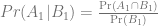
to compare to

What we observe (or can observe) are , , and , where (for example)

and so forth. Now, the probability

for example, gives us

Repeating that, we see that the probability that we need is given by

This is because our outcomes are clearly defined: they are mutually exclusive, and they are exhaustive – i.e.

Same for B₂. Thus will we get the two numbers that need to answer the questions: (1) what was the probability of getting tickets conditional upon being a Miley Cyrus Fan Club member; and (2) was it greater than the probability of securing tickets conditional upon not being a fan club member? I should point out here that the tricky part of this is going to be finding A₂ and Pr(A₂ ). Less so, perhaps for members of the Miley Cyrus Fan Club than for the general population. The value of that information will make a very big difference to our conditional probabilities: what if, for example, they are different numbers, but very similar numbers? How different do they have to be? Enter the (pronounced ky, to rhyme with sky) test for independence.

Chi-squared

The test for independence will test for us the null hypothesis (the default hypothesis) that , versus the alternative that . For this we need all four possible joint observed cells:

If the two probabilities are in fact equal, then we would expect to see (for example):

Then we calculate our test statistic:

(This equation refuses to convert. I’ll fix it later). Here you go (anyone want to explain why the equation beats the WordPress renderer?):

I.e. the sum of the squared values of the (observed – expected) cells for each of the two outcomes. This could also be done the other way around, or using the Tickets columns, rather than the Membership rows. With n – 1 = 1 degree of freedom, we just need that statistic to be greater than 3.84:

to reject our null hypothesis and conclude that the distribution of ticket-getting was in fact different for Miley Cyrus Fan Club members than for non-members. If the members had a higher conditional probability of securing tickets then, again, there is no case. If they are not statistically significantly different, they’ve been ripped-off. Again, whether they should have known this beforehand is a matter for a jury: we just do the numbers.

Done? Not even close. What if there was more to it than that?

Regression

Regression analysis: regression analysis will offer two distinct advantages in this instance; one for the prosecution, and definitely if the defence has demonstrated, above, than Miley Cyrus Fan Club members did in fact get a better deal on tickets than non-members, and one for the defence, for the same reason:

1. Regression analysis will be able to quantify the degree to which being a member of the fan club increased the probability of securing a ticket to the show(s).
2. Regression analysis will be able to identify the statistical significance of the relationship between fan club membership and ticket-securing, controlling for other factors.

Our regression model appears thus:

Keeping it simple Ordinary Least Squared. That is part (1): this model will positively identify whether being a member of the fan club (a dummy variable: 0 = not a member; 1 = member) affects the probability of securing tickets. For purposes of compensation, it will also quantify the degree to which that probability increased (if it increased at all).

However. What if there was some other difference? We know, for example, that scalpers landed on these tickets like (insert joke here – who don’t you like?). Suppose Miley Cyrus Fan Club members differed in some specific other respect? Perhaps they just didn’t log on as quickly? Do they have a slower connection? Was a child doing it with their parents credit card (the assumption being that they were slower to manoeuvre the system)? On to multiple regression! Controlling for these factors, our model becomes:

The more statistically significant explanatory variables we introduce into our model, the less statistically significant (and, probably, economically significant) will become, and the weaker will become the class action lawsuit against the Hannah Montana people.

Seems like a waste of perfectly good econometrics/statistics, one might think. The suit will probably contain every fan club member who did not get a ticket, though, asking for triple damages plus legal fees. I reckon it’s worth the effort for the companies being sued.

I keep telling my students that econometrics can do everything…

HowTo: Reporting bias. Or, why do little kids prefer apples from McDonald’s?

The story:

“McFood” Better Than Food, Kids Say

Robinson and colleagues studied 63 low-income children enrolled in Head Start centers in California. The kids ranged in age from 3 years to 5 years.

Told they were playing a food-tasting game, the kids sat at a table with a screen across the middle. A researcher reached around either side of the screen to put out two identical food samples: slices of a hamburger, french fries, chicken nuggets, milk, or baby carrots.

The only difference between the pairs of food samples was that one came in a plain wrapper, cup, or bag, and the other came in a clean, unused McDonald’s wrapper, cup, or bag. The kids were asked whether they liked one of the foods best, or whether they tasted the same.

I love the idea of some brainless reporter going ‘newspaper’ with the heading, yet still using the word “kids”, rather than, say, “children”.

The results of the study!

• 77 percent of the kids said the same french fries, from McDonald’s, were better in a McDonald’s bag than in a plain bag (13 percent liked the ones in the plain bag; 10 percent could tell they were the same).
• 61 percent of the kids said milk tasted better in a McDonald’s cup (21 percent liked milk in a plain cup; 18 percent could tell it was the same).
• 59 percent of the kids said chicken nuggets tasted better in a McDonald’s bag (18 percent liked them in a plain bag; 23 percent could tell they were the same).
• 54 percent of the kids said carrots tasted better in a McDonald’s bag (23 percent liked them in a plain bag; another 23 percent could tell they were the same).
• 48 percent of the kids liked hamburgers better in a McDonald’s wrapper (37 percent liked them in a plain wrapper; 15 percent could tell they were the same).

Now, I’m vegan, so my familiarity with old whatshisarches is a little rusty – but aren’t hamburgers their business? To add context:

Kids who preferred “McFood” tended to live in homes with a greater number of television sets and tended to eat at McDonald’s more often than kids not influenced by the McDonald’s brand name.

I’m not surprised the study got that the right way around, but I am pleasantly surprised that the reporter kept it so. The rest of the article goes on about marketing. Apparently McDonald’s provides parents with the “safest food” – whatever that is supposed to mean.

Now, here’s the problem. The results of this study are potentially two things, and probably a mixture of both. The first thing, the phenomen being measured and presumed to have been found, is revealed preference. For all that economists draw demand curves and insist our neo-classical models explain the world, one cannot actually measure demand, only consumption. Thus we need to measure revealed preferences, rather than preferences directly. Hence, little children are revealing a preference for foods in McDonald’s wrappers.

Here’s the thing, though. The children are tasting the food, then saying which they thought tasted nicer, as opposed to selecting one (in which case the preference for McDonald’s brands would be revealed). If the food is the same, this is irrational, but there’s a slight difference in what’s being measured and what we are concluding:

Children do not necessarily like milk better given that it is in a McDonald’s container, they just say they like it better given that they have seen it in a McDonald’s container.

That is, we aren’t measuring what the children like, but what they say they like. This exposes their responses to reporting bias. I’m a health economist, so I find this in that context. I give you reporting bias in Self-Assessed Health.

Self-Assessed Health (or SAH) is how health is often measured. It’s too damned expensive to have every respondent in the Medical Expenditure Panel Survey see a doctor. So our surveys ask something like, “how would you rate your own health?”, and give you, as options, “Very Good”, “Good”, “Fair”, “Poor” and “Very Poor”.

Now. Suppose the question did not specify that you consider only people your own age, income bracket, choice of sport (NFL players?), etc.”

• My grandparents are in their mid-80s. My grandmother has had, I think, everything replaced one can have, without having had plastic surgery. Compared to their friends, however, my grandparents both rate their health as very good. If you or I (assuming you aren’t 80, while reading this) had their health, we’d think otherwise.
• Poor people will rate the same level of health as better for them than a rich person – because their expectations are different.
• A diabetic might rate their health relative to their disease state. So they will say their health is Good, while we think, “Dude – you’ve lost a leg!” Again, different health-expectations.

This is reporting bias. Two excellent papers on this (full disclosure: both include as co-authors attractive former colleagues, and one my PhD supervisor): Reporting Bias and Heterogeneity in Self-Assessed Health. Evidence from the British Household Panel Survey; and Does Reporting Heterogeneity bias The Measurement of Health Disparities?. I remember the latter very well because using “bias” as an active verb always struck me as a little wobbly. But like I said, the colleague is very attractive. There are different standards for pretty girls (I’m incredibly superficial).

When is reporting bias a problem? If one is modelling health care demand, health insurance purchasing, etc., it is not that much of a problem. People consume according to their perception of their needs. If their perception is wrong, that’s their misfortune; only that the link between what they think they need and what they purchase is properly measured. If, on the other hand, one is modelling inequalities in health, then it is that much of a problem. As above, if a poor person rates a given level of (relatively low?) health higher than a rich person, measuring income-related inequalities in health becomes very tricky indeed. Same for international comparisons.

The latter of the two papers to which I linked is a good starting point, if you’re interested. It explores the use of anchoring vignettes to get some standard comparators in terms of health, and see how different ages, genders, incomes, nationalities affect the rating of that given health state (identified descriptively in terms of mobility, pain, etc.), and then use those as ‘handicaps’, to correct for bias in individual responses. It works fairly well.

Back to the story of the children and the clown! How sophisticated are little children, anyway? How much of a game might they be playing? Are they honestly saying, “I like this better because of the brand, and because I’m wilfully irrational”? I say this because, absent the surrounds of a McDonald’s restaurant, I don’t see how a wrapper in isolation can increase utility (in which case it might not be irrational, although it still does not affect the taste).

Might they also be saying, though, that they like the food wrapped in McDonald’s paper because they remember McDonald’s food as tasting better than other meals, including home-cooked? Following that, might they also be saying they liked it better in the hopes that their rating will get them more McDonald’s food in the future?

I submit that both are very possible. Children are certainly sophisticated enough to play their own games in a study like this one. Remember also the socio-economic gradients tentatively identified amongst the children. Split them up poor/wealthy, and imagine the food that their households consume from a supermarket, the other places they might eat, etc.:

• Odds are, the wealthier families are having better ingredients (even down to, say, frozen food) end up on their plate, so that the disparity between home-cooked and McDonald’s cooked food is greater.
• There is also potentially an exposure effect – wealthier children being exposed to a greater range of non-home eating, including proper restaurants. This would devalue the association with McDonald’s.
• In terms of the memory of a preference for McDonald’s, even the environment in which they eat is a potential factor. For a relatively poorer child, McDonald’s is nicer than his home, perhaps. Not so for a wealthier child, who may even have McDonald’s brought home, more than in a restaurant.

See? Reporting bias. Ultimately I’m saying this study is information that should be considered in a wider context. It doesn’t simply mean that McDonald’s is winning some war against parents, or that McDonald’s will be worse than ever, now that it thinks it can market milk and carrots successfully. Alternatively it is, and we should be thinking about socio-economic gradients in consumer behaviour of this type (it’s not really my area of health economics).

For me, McDonald’s will always be the back-up public bathroom if I can’t find a Starbucks. I heart New York.

HowTo: Propensity Score Matching

Sadly, Billy Bragg never wrote a song about Propensity Score Matching (although his Walk Away Renee might do, in a pinch?).

I give you this not because it is of great use or importance (or, to be fair, even interest), but because I’m looking into it for purposes of my own. And misery loves company. Suckers. So this is not a ‘how to’. I’m not even the first person to write about it on a blog. Consider it more of a ‘what is’. Without the maths, even.

I’ve mentioned the evaluation problem previously. I’ll illustrate with an example upon which I’ve worked previously: hysterectomy (NB: I’m not one of those authors). Simplifying that problem a bit, suppose there are two types of hysterectomy: Abdominal, and Vaginal (fellows: a hysterectomy is the removal of the uterus). The evaluation problem is this. You cannot give the same woman both types. Once you’ve given her an Abdominal hysterectomy, that’s it (fellows: women only have one uterus. What?). She cannot have a Vaginal one. There is no perfect counter-factual information with which to compare the factual.

Ergo you cannot compare the effectiveness of two types of hysterectomy on exactly the same person. This is also know as the effect of treatment on the untreated. This is where clinical trials come in. A Randomised Control Trial is one where all participants have been randomly allocated treatment or non-treatment (or Treatment A, Treatment B, etc. You get the picture). The idea is that the pool of treated patients is exactly the same as the pool of untreated patients. More importantly the probability of being treated, given any personal characteristics you might have, should be exactly the same as the probability of not being treated (and vice versa: the probability that you’re a male, for example, given you were treated, should be exactly the same as the probability that you’re a male given you weren’t treated – assuming treatment was not a sex-change operation. That really was beneath me).

Now it gets interesting. This is all well and good for clinical trials, but something else exists – something called a natural experiment. A natural experiment for our purposes is one without a properly-constructed control group, and usually arises with retrospective data analysis. If you wanted to examine something pertaining to an outbreak of Ebola Zaire, you can hardly randomise villages in central Africa, giving some of them Ebola and others not. If it so happens that you do have delusions of Dr. Mengele, kindly keep them to yourself. Nor, if any outbreak happens to occur, can you easily find a control group – no other region will be exactly alike in terms of culture, climate, etc. and there’s no guarantee that if you use the same region at an earlier period you will be successful (you could have missed the famine or war that led to young men eating a gorilla that was found dead rather than shot, or however the outbreak started).

An example I’ve also used in class is so-called 9/11 (no, I’m not disputing it happened, Americans just have a thoroughly backwards approach to dates. The American 9/11 was actually our 11/9 and it is the Americna who are wrong. I’ve also been to ‘ground zero’ and discovered a truly disgusting entrepreneurial spirit at work. Perhaps more on that another day, but I doubt it. It makes me want to throw up). It is a perfect natural experiment for emergency services responsiveness – but not one that can be carried out under RCT conditions, for obvious reasons.

Now, non-experimental data is likely to contain biases of one kind or another. In health care, for example, we cannot simply look at the health care demand of insured vs. uninsured people – the very fact that an insured person is insured means they will/may

(i) use more health care because there’s a co-pay, or some other deduction, and/or

(ii) use more health care because they’re sicker, which is why the bought the bloody health insurance in the first place, or

(iii) use more health care because they are more educated and make more money, hence can afford health insurane and understand the benefits of investments in their health stock (this last category consists entirely of Michael Grossman).

This is known as selection bias. And it can be passive or active, if you like. If you conduct a survey in only, say, the north of Italy, you get selection bias. Because is more health, wealthy, educated and industrialised than the south. If you conduct a survey on Fox News, you get self-selection bias, because only viewers of Fox News will respond. So you can’t compare teaching in public/private schools using test scores, because there will be systematic (non-random) differences. You can’t compare an outbreak of Ebola in Central Africa with no outbreak in West Africa. You can’t compare emergency response to a terrorist attack in New York to one in London or Madrid for the same reason.

There is also simultaneity bias, or reverse causation. That is to wit (I’m old-fashioned), consider this: does greater litigiousness generate more litigation lawyers, or did more litigation lawyers generate more litigation? Some of both, no doubt, but a regression model needs to be built to pick up causation in the right direction.

So, Propensity Score Matching. This is an econometric technique for use with non-experimental data. It is designed to overcome the bias that you will face if and when you decide to compare the effects of treatment on the treated with those of non-treatment on the non-treated, if you get your data from outside an RCT setting. If your treated and control groups are from different areas, different datasets, different time periods, and so forth. Propensity Score Matching is also not the only approach. Follow the link for non-experimental data, and you’ll find a handful more. The elsblog discusses some, as well.

The seminal paper for this stuff, by the by, is Propensity Score-Matching Methods For Nonexperimental Causal Studies by Rajeev Dehejia and Sadek Wahba (he’s from Morgan Stanley – no webpage).

So the trick is matching. Using covariates (Age, Gender, Income, Education, Marital Status, Hair Colour – anything of economic and/or statistical importance to the outcome of interest), we can theoretically break our sample of treated people into groups, or bins. All single males 28 years old, college-educated, non-smoking, living in urban environments, and so forth can then be compared, in terms of treatment, only with other single males 28 years old, college-educated, non-smoking, living in urban environments, and so forth. Repeat. However, see the problem? Every bin needs a corresponding bin in the non-treated group (this could be another sample). If there isn’t one, you have to exclude all of those people. If there is, but the bin is not sufficiently populated, so too out it goes.

The trick, the goal, the purpose of Propensity Score Matching is overcoming the problem of dimensionality. Comparing treated individuals to non-treated with non-experimental data is an enterprise entirely victim to the covariates at hand. Suppose you have 15 econometrically relevant explanatory variables. To employ them all is to render the econometric problem practically unsurpassable, but to use only, say, 5 of the variables will render the estimation and explanation of the response variable practically useless. Propensity score matching does this: it is a matching method that, instead of using every X_i, uses p(X_i), where p(X_i) is the probability of having been treated, given the covariates. The probability p(X_i) is the propensity score.

Bingo! Our dimensionality problem is gone. Instead of n covariates, we have a single score.

Then, each treated individual (assuming for the sake of argument that it is an individual with whose treatment we are dealing) is compared to non-treated individuals according to their propensity score. There are a few approaches to this, too. First, the treated individuals have to be ranked. They can be ranked in ascending order, descending order (this is with respect to their propensity score) or randomly. The ranking determines the order in which they are matched.

Once ranked, they are matched. Individuals can be matched with replacement or without replacement. Without replacement, once a non-treated individual has been matched, or ‘paired’ with a treated individual, they are removed from the pool. This can be a problem if you don’t have loads of non-treated individuals, as each subsequent match may involve greater distances (also in terms of the propensity score). Moreover it may not make sense. If you do use RCT data, comparing means (or using regression), you still compare with replacement, effectively. It should be case-by-case, but for me the arguments for matching with replacement are convincing enough.

Next: how many matches? If you match strictly one-to-one, you guarantee minimum bias, and minimum ‘distance’ between matches. But if you use more matches, you should get more precise estimates, albeit at the risk of greater bias (like the with/without replacement. As this propensity score ‘distance’ increases, so does the likelihood that you are comparing a treated individual with a systematically different non-treated individual). There are a couple of algorithms for this. One is the nearest-neighbour method, which automatically takes the m nearest non-treated propensity scores (but you pick the m – although that too can be optimised), and another is the ‘caliper’ method, which picks however many non-treated individuals are within a pre-specified ‘distance’ (that too could be optimised). This is also a case-by-case concern. There is no set rule for applying the Propensity Score Matching method to non-experimental data.

The Dehejia and Wahba (2002) paper uses data from a preceding paper by Robert LaLonde, comparing training programmes. This gave them the advantage of having on hand experimental data with which to compare results from a constructed non-experimental problem. Their results were pretty good, and Propensity Score Matching has entered the methodological world.

Why of interest to me? I intend, along with a colleague, in applying some Bayesian value-of-information standards to the method, to look at some of the preliminary testing that goes on to assess the suitability of comparison groups, as well as to evaluate the likelihood that the ultimately-estimated Treatment Effect is correct for a given individual. Look out for future posts containing discussion of value-of-information analysis. Now that stuff is fun.